Office Q&A: Random time values, conditional formatting, and a PivotTable solution


This month, I received a lot of Excel questions. So in this article, we'll tackle random time values, an icon-displaying conditional expression and format, and a quick PivotTable solution. For your convenience, you can download the example .xls and .xlsx files. This article uses Excel 2007, but there are no significant differences between Ribbon versions. I haven't included 2003 instructions, but the only difference will be menu choices versus ribbon options.
Random time values within a range
Terence wants to generate random time values within a specific time range. Fortunately, this task isn't as difficult as it initially sounds. Using RAND() and several time functions, you can easily accommodate this requirement.
The first thing you need is a start and end time; be sure to apply the Time format to both cells. At this point, you might consider two functions: RAND() and RANDBETWEEN(). The latter won't work, at least not easily. It evaluates integers, and time values are stored as decimal values. Figure A shows the ABS() function being used to return the decimal value of each time value. You don't need the ABS() function for this solution, but it helps clarify what we're doing. If you think about it, the .5 for noon makes perfect since. Noon is halfway through the day.
Figure A

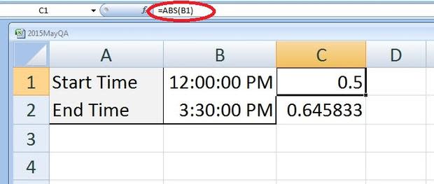
Enter a start and end time.
Because we're evaluating decimal values, we'll use the RAND() function in a simple expression in the following form:
=RAND()*(end-start)+start
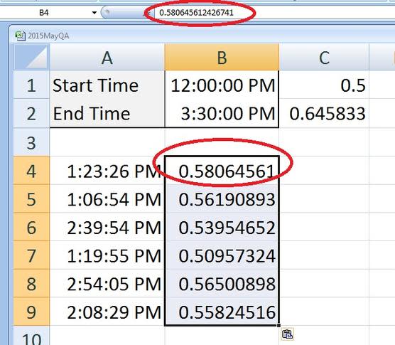
Figure B shows the results of entering this expression in D4 and copying it to several cells:
=RAND()*($B$2-$B$1)+$B$1
As you can see, the expression returns random decimal values between the values of .5 and .645833.
Figure B
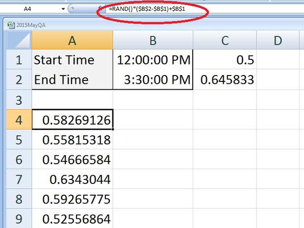

Enter the RAND() expression.
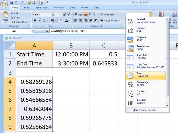
But Terence wants to see time values. Thanks to the ABS() function we discussed earlier, you already know that those random decimal values represent time values. To display the decimal values as time values, do the following:
Select D4:D9.
In the Number group on the Home tab, click the Number format dropdown and choose Time (Figure C).
Figure C

Once you change the format, the decimal values display time values, as you can see in Figure D.
Figure D

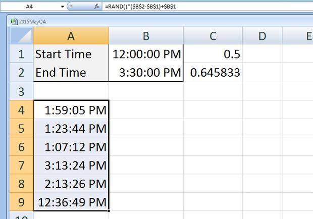
Choose the Time format to display time values.
The random values might repeat, but they will fall within the start and end time range. The RAND() function evaluates every time you change your sheet, so working with a RAND() function or expression can be difficult. You might find it easier to copy the values to another location using the Paste Special command as follows:
Select A4:A9 (the RAND() expressions).
Press [Ctrl]+C to copy the expressions to the Clipboard.
Select a target cell such as B4.
From the Paste dropdown (in the Clipboard group on the Home tab), select Paste Values (Figure E).
Figure E
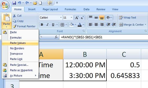

This feature pastes the values, as shown in Figure F, instead of the expressions used to evaluate them.
Figure F

Work with the values, not the RAND() functions.
A conditional icon set
Cristin wants to use the 3-arrow icon set to denote a change in rank between two columns of text values. Unfortunately, there's just no easy way to get what Cristin wants because the icon set evaluates a single column of values. Cristin has two columns of text values. Sometimes it's easier to change the sheet's structure than it is to force a feature to work within the existing structure. This might be one of those times. (Excel 2003 doesn't support this feature.)
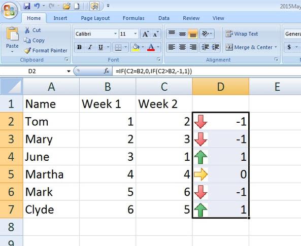
Figure G shows a simple representation of Cristin's sheet; Excel's icon set can't evaluate the text values. It also shows a new structure using numbers instead of text values. I've simply transposed the structure; instead of repeating text values by their ranked value, I entered the numeric rank for each text value. The icon set can't accommodate two columns either, so I added a helper column using a simple comparison expression and copied it accordingly:
=IF(C2=B2,0,IF(C2>B2,-1,1))
Figure G

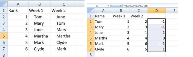
Restructure the data.
This expression has three conditions:
If the two values are equal, the expression returns 0.
If the value in column C is greater than the value in column B, the expression returns -1.
If the value in column C is less than the value in column B, the expression returns 1.
In other words, if the two values are equal, the ranking is the same in both weeks. When the value in C is greater, the ranking has gone down; a higher value in B means the ranking has improved.
Now we have a column of values that the icon set can evaluate, so the next step is to apply the conditional format to column D as follows:
Select D2:D7.
On the Home tab, click Conditional Formatting in the Styles group.
Select Icon sets from the dropdown, and then choose the 3 Arrows Colored option (Figure H) to see the results shown in Figure I.
Figure H
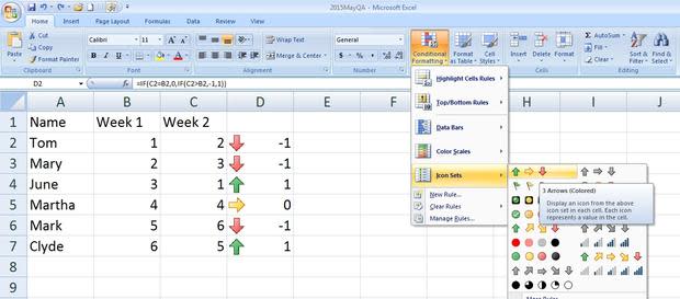

Figure I

Excel displays conditional icons.
If you want to hide the values, repeat steps 1 and 2 above and do the following:
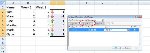
From the dropdown list, choose Manage Rules.
In the resulting dialog, choose the appropriate rule if necessary and then click Edit Rule (Figure J).
Figure J

In the bottom-right corner, check the Show Icon Only option (Figure K) and click OK twice. Doing so will hide the evaluated values, as shown in Figure L.
Figure K

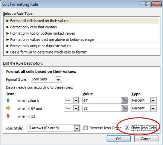
Figure L

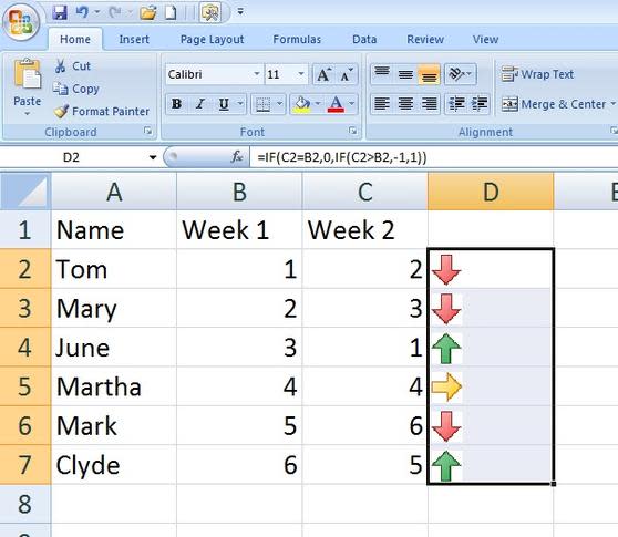
The format displays only the arrows.
You've learned a bit about the built-in icon set and what it can and can't do. Unfortunately, Cristin still doesn't have a solution that's easy to update. While this solution works, restructuring data isn't easy. Another problem is accommodating new ranking values each week. If you insert a new column, the formulas continue to evaluate columns B and C. You can copy the expressions to the right, freeing up a column for the new week's values, but you'll have to clear the conditional format from column D. More important, you'll have to do this every week. You could create a macro to do it for you, but I'm not convinced that there isn't a slicker way (without code) to implement this solution. Please share your own ideas in the comments section.
PivotTable counts unique values by group
Lan tracks the number of times a nurse is called and each nurse can be called multiple times on the same day. She'd like to count the number of unique dates for each nurse. A PivotTable is the most efficient solution for Lan, but the dataset needs a grouping value before the PivotTable can work.
We'll work with the simple data set shown in Figure M. As you can see, Lan and Lucy have multiple entries and many are duplicates. We're not concerned with the duplicates, so we don't need to complicate the example any further.
Figure M

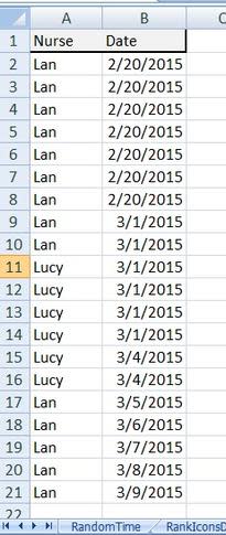
We'll use a PivotTable to count the number of unique dates for each nurse.
The first step is to add a rather complex expression to the data set as shown in Figure N. Add the following expression to C2 and copy it to C21.
=IF(SUMPRODUCT(($A2:A$21=A2)*($B2:B$21=B2))>1,0,1)
Figure N

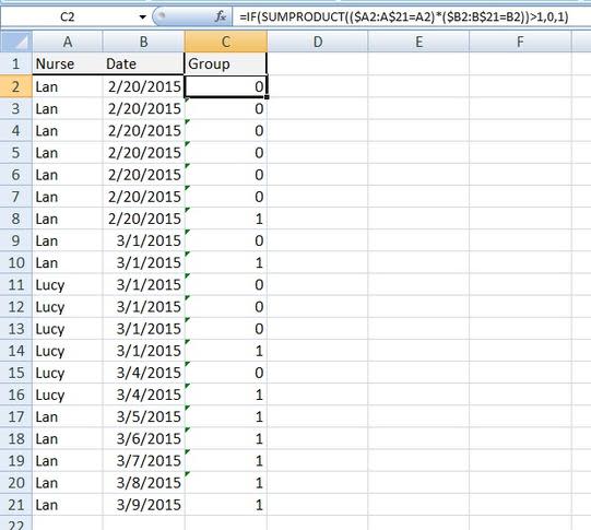
This expression returns a column of 0s and 1s.
In a nutshell, this function counts the number of unique occurrences for each nurse. Although Lan was called seven times on 2/20/2015, the function returns only one 1 for that date. Now, let's generate a PivotTable based on this data, as follows:
Click any cell in the data set.
Click the Insert tab and click PivotTable in the Tables group.
In the resulting dialog, click OK to create a new page. If you want to insert the PivotTable in the current sheet, select the Existing Workshop option and select an anchor cell (Figure O) before clicking OK.
In the PivotTable Field List pane, drag Nurse to the Row Labels section.
Drag Group to the Values section, which defaults to a sum function (Figure P).
Figure O

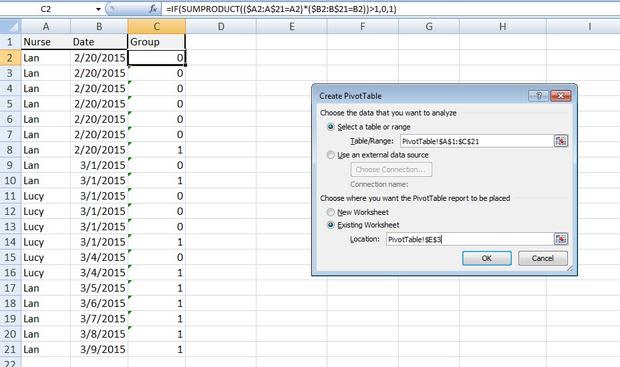
Figure P
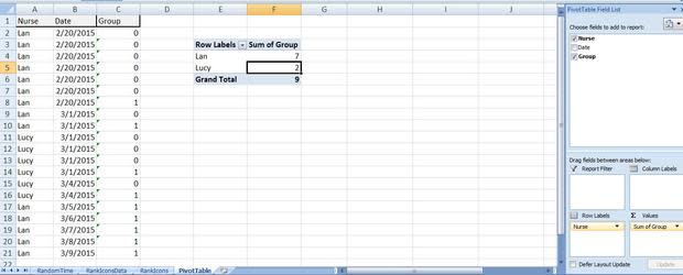

Lan has seven unique call days and Lucy has two. If you're using Excel 2003, you can skip the additional function and use the PivotTable's Distinct Count function.
PivotTables make quick work for evaluating grouped values. The one drawback is that you must update a PivotTable when you change the underlying data. To do so, click inside the PivotTable and click Refresh in the Data group on the contextual Options tab.
Send me your question about Office
I answer readers' questions about Microsoft Office when I can, but there's no guarantee. When contacting me, be as specific as possible. For example, "Please troubleshoot my workbook and fix what's wrong" probably won't get a response, but "Can you tell me why this formula isn't returning the expected results?" might. Please mention the app and version you're using. I'm not reimbursed by TechRepublic for my time or expertise, nor do I ask for a fee from readers. You can contact me at susansalesharkins@gmail.com.
Also read...
How to generate sequentially numbered documents using Publisher
Three ways to return the average age for a group using Excel
Office Q&A: Word field codes, Excel values, and conditional formats
Two quick graphic tricks that return big results in a Word document
